Controlled-Release Experiment to Optimize Emission Quantification of H2 Point Sources
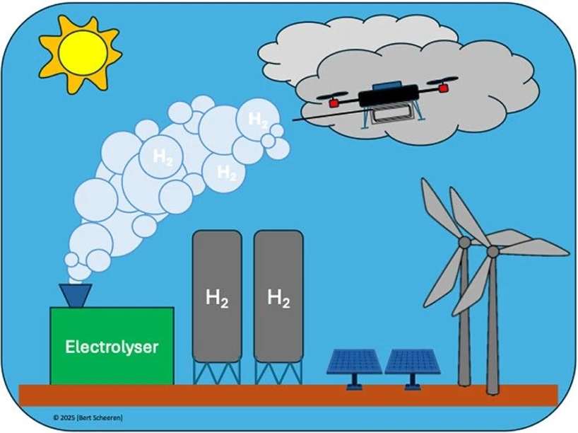
ACS EST Air 2026, 3, 6, 1576–1585: Graphical abstract
This study optimizes the quantification of hydrogen point-source emissions through controlled-release experiments using an 8 kW electrolyzer. A multiplatform AirCore sampling system coupled with a high-resolution GC-PDHID simultaneously measured hydrogen, methane, and carbon dioxide to evaluate how sampling conditions influence emission estimates.
Analysis of UAV and ground-based measurements showed that plume coverage, wind variability, and sampling resolution strongly affect emission accuracy. The results also demonstrated that hydrogen plume behavior closely resembles methane, indicating that established methane monitoring strategies can be adapted for hydrogen leak detection and supporting future assessments of hydrogen as an indirect greenhouse gas.
The original article
Controlled-Release Experiment to Optimize Emission Quantification of H2 Point Sources
Iris M. Westra*, Hubertus A. Scheeren, Mareen J. Penninga, Steven M.A.C. van Heuven, and Harro A.J. Meijer
ACS EST Air 2026, 3, 6, 1576–1585
https://doi.org/10.1021/acsestair.6c00006
licensed under CC-BY 4.0
Selected sections from the article follow. Formats and hyperlinks were adapted from the original.
Currently, more than 90% of hydrogen produced is gray hydrogen, derived primarily from steam methane reforming or coal gasification, both of which are carbon-intensive. (1) Considering the global hydrogen budget, the primary natural source of atmospheric hydrogen is sunlight-driven production (e.g., via methane oxidation), contributing 38 ± 6 Tg yr–1 (about 55% of the total budget). The largest anthropogenic source of hydrogen is the combined contribution from biofuel burning and wildfires, amounting to 12 ± 4 Tg yr–1. (1) Hydrogen’s indirect Global Warming Potential (GWP) leads to the lengthening of the lifetime of CH4 and ozone, and to increased levels of stratospheric water vapor (H2O). (2,3) As a result, the GWP of H2 over a 100-year time scale has been estimated at 11.6 ± 2.8, indicating that H2 is 12 times more potent than CO2. (4) While this is about half the GWP of CH4 it underscores the significance of hydrogen’s indirect effects on climate when released into the atmosphere. (5) Until recently, small but climate-relevant hydrogen emissions remained undetected along the entire hydrogen value chain. However, such hydrogen losses during production, transport, storage and consumption could lead to a greater atmospheric hydrogen burden. (3) To illustrate the impact of hydrogen leakage, the HC2017 scenario presented in Hauglustaine et al. (2022) shows that, for a hydrogen mix of 30% blue (gray+CCS) and 70% green hydrogen (renewables) with leakage rates of 1–3%, the climate benefit is substantially reduced, with hydrogen CO2-equivalent emissions corresponding to 20 to 54% of the avoided CO2 (based on GWP100 and GWP20, respectively). At higher leakage rates (>10% for a 100-year horizon; > 5% for a 20-year horizon), this hydrogen mix results even in a net climate penalty, where CO2-eq emissions exceed the avoided CO2.
Thus, far, current loss rate estimates, ranging up to 10%, are solely based on bottom-up emission estimates (i.e., theory-based). (6−8) A limited amount of suitable measurement equipment and a current lack in actual measurements causes these estimates to have no validation. (9)
Only recently, sensitive new techniques to detect low-level hydrogen emissions along the value chain on an atmospheric scale have become available. In our previous study (10) we combined an established high-precision analysis method (gas chromatograph─pulsed discharge helium ionization detector; GC-PDHID) with a newly applied sampling method (active AirCore (11)) deployed from various mobile platforms, to detect significant hydrogen emissions originating from a chemistry park in the Netherlands. (10) In the meantime, Aerodyne Research Inc. (USA) has developed a laser-spectroscopy-based instrument with which atmospheric hydrogen can be measured continuously, through oxidation to water vapor and a subsequent optical measurement, achieving ∼5 ppb precision (per 5 s). (12,13) The Norwegian oil company Equinor, in collaboration with Advanced Monitoring Solutions (AdMS) and the Department of Chemistry (University of Oslo) in Norway, have developed a mass spectrometer system capable of measuring small atmospheric hydrogen mole fractions (<1 umol mol–1 i.e., ppm) with a detection limit of ∼10 nmol mol–1 (i.e., ppb) directly from dried ambient air. (14) Hence, with these new developments in atmospheric hydrogen detection techniques, the hitherto unknown hydrogen emissions along the hydrogen value chain become visible.
In the field of emission quantification there is already a wealth of reported experiments for greenhouse gases (GHG), like methane (CH4), (15) with the aim of making emission quantifications more reliable and accurate. These emission estimates help reduce uncertainties in bottom-up estimates of the greenhouse gas (GHG) budget. (16)
Optimal airborne plume sampling for methane emissions from a point source depends on factors such as the downwind distance, maximum flight time, measurement precision, and atmospheric stability conditions. (17) Especially during near-source sampling (<500 m downwind), accurate visualization of the plume in both the horizontal (width) and vertical (height) plane is critical for reducing significant discrepancies between measured emissions and inventory estimates. (18−20) Furthermore, Morales et al. showed that measurement uncertainties increase primarily under conditions of wind speeds below 2 m s–1, wind direction variability greater than 33°, and sampling at downwind distances greater than 75 m. So far, under the most favorable measurement conditions, CH4 emissions could be quantified with an overall uncertainty of at best 30%. (17)
In this study, we use measurements from a controlled-release experiment to optimize the quantification of hydrogen point-source emissions by identifying the most influential parameters contributing to uncertainties in the emission estimates.
In the following, we first outline the sampling and analysis techniques, building on Westra et al., (10) after which we give a site description and further necessary prior information. The observations obtained from ground-based and airborne measurements are analyzed using a Gaussian plume dispersion model combined with a Monte Carlo uncertainty analysis to estimate the emission rate. At the end of the paper the conclusions and outlook on our methodology will be given.
2. Materials and Methods
2.4. Analysis Methods
The Agilent 8890 gas chromatograph pulsed discharged helium ionization detector (GC-PDHID) system setup was designed for the precise and accurate analysis of H2, CO2 and CH4 in dry ambient air. We chose a PDHID for its high sensitivity, reliability, and good linearity from low to high mole fractions for H2 (here typically ranging between 0.5 up to 5 ppm). The system setup enables, via a heart-cutting procedure (forward-flush mode of the O2 and N2 fraction), the simultaneous detection of CO2 and CH4, which can aid in the source apportionment of atmospheric H2.
Our system design was partly based on the Agilent setup 7890–0237 “Impurities in Monomers Analyzer by PDHID” and a GC setup by Wang et al. (24) The PDHID system uses Helium 5.0 (99.9999% Vol. %, Westfalen) as carrier gas, for a combination of a HayeSep Q, (G3591–81004, 6 ft,
3. Results and Discussion
3.2. AirCore Results
The determined emission rates were achieved by applying the Gaussian dispersion model to the found H2 enhancements for each transect, and by taking into account the atmospheric conditions during sampling, following the approach outlined in Westra et al. (10) Using an 8 kW electrolyzer (Figure 4) with a known, continuous release rate of 1.1 ± 0.1 m3 h–1 as a controlled source, we analyzed 14 data sets to determine a mean weighted hydrogen emission rate of 0.94 ± 0.06 m3 h–1. This agrees well within uncertainty with the known source rate. The relative uncertainty (ratio of uncertainty over average) of the emission estimate is 6%, compared to 9% for the known source. The source-based uncertainty was derived from variability in the electrolyzer exhaust monitored over multiple hours. More information with regard to the uncertainty analysis can be found S1.5. All data gathered during the field experiments is given in Sections S2.1 and S2.4.
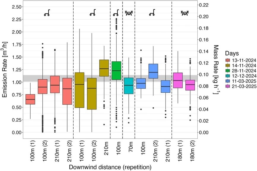 ACS EST Air 2026, 3, 6, 1576–1585: Figure 4. Emission rates estimated for six sampling days using the Gaussian dispersion model and the AirCore technique, measured downwind of the electrolyzer at varying distances. Measurements were conducted either at ground level (cart icon) or via UAV (drone icon). Boxplots represent results from 500 Monte Carlo simulations, displaying the mean and interquartile range. From 28 to 11–2024 onward the, as described, an optimized sampling method was used.
On day 13–11–2024, the quality of the data collected along the first 100 m trajectory was lower due to a sampling flow rate of ∼45 sccm combined with a relatively high rate of displacement. As a result, the full plume width was not captured, and the spatial resolution of the measurements was insufficient. This limitation, consistent with the findings of Mohammadloo et al., (15) led to the underestimation of the actual emission rate. Particularly for transect 100 m (1), where the plateau-shaped peak approximated a Gaussian peak, led the dispersion model to substantially underestimate the emission rate (Sections S1.6 and S2.3). Furthermore, the relatively large spread in data points observed throughout the remaining trajectories of 13–11–2024 can be attributed to the sampling time of the experiment, during which the atmospheric variability (i.e., wind speed and direction) impacted the uncertainty. As a result, the Monte Carlo simulations produced a wider range of solutions due to this variability, and thus a greater spread in the values. So, the impact of the atmospheric conditions could be reduced by minimizing sampling time and thereby reducing the atmospheric variability.
For day 14–11–2024 (Figure 5), an average wind speed of 1.7 ± 1 m s–1 was measured. According to Andersen, (22) wind speeds below 2 m s–1 lead to ill-defined wind directions, making the plume less likely to follow a stable path and thereby increasing uncertainty in the emission estimate. Hence, it is likely that the lower wind speed on this day contributed to less reliable results in the emission quantification. Moreover, for day 14–11–2024, the wider spread observed in the estimates (Figure 4) is attributed to incomplete coverage of the plume width along the 100 m downwind transects.
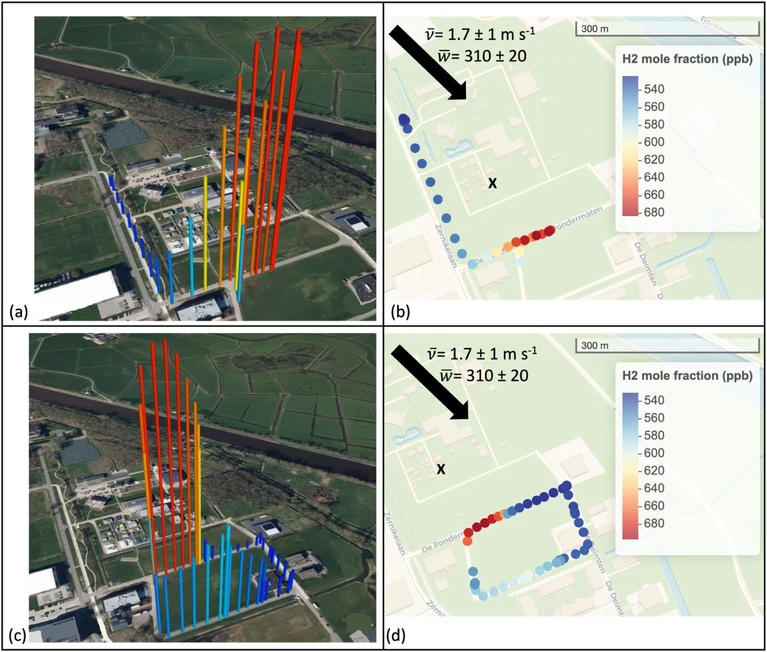 ACS EST Air 2026, 3, 6, 1576–1585: Figure 5. Trajectory of ground-based AirCore profile downwind of the electrolyzer (shown by the “x”) on 14–11–2024, first round (a, b) and second round (c, d), shown on a 300 m scale and the H2 mole fraction (ppb) given in the legend on the right. The total sampling time of the trajectory was 35 min. Map tiles © Mapbox, data © OpenStreetMap contributors (ODbL), modified by the author.