Leveraging Local Libraries for Positively Parsimonious Peak Tables (James Harynuk, MDCW 2026)

🎤 Presenter: James Harynuk (University of Alberta)

💾 PDF presentation

Abstract

GC×GC- MS shines when doing non-target analysis, and is an incredibly important tool for studying human health, human exposures to exogenous compounds, and transformations of compounds released into the environment. The enhanced separation and expanded separation space permits us to deliver very pure peaks to the mass spectrometer, free from many coelutions and also free from bleed from the primary column. This pure peak then results in a much cleaner, high quality mass spectrum, regardless of the mass spectrometer used. If a high resolution mass spectrometer is used, we then know the exact mass (and thus elemental composition) of every ion in the spectrum. 

This is a truly important tool for studying these problems. The inspiration for this work lies in the problem of what to do with unknown unknowns – those compounds not in any library? We have been exploring new, simple ways to improve the consistency in our reporting of compounds in non-target analyses. Using a combination of a user library and relatively simple tools, we can ensure that we always recognize the same compounds across various samples and sample types, even if we do not know exactly what the compound is. This should improve the quality of downstream data analysis, and potentially help standardize some of the tools used in GC×GC-MS data processing.

Video Transcription

Today I want to talk about some of the ideas we’ve been exploring to improve our data quality. The theme is a bit unusual: down is the new up — in other words, simplifying some parts of the workflow can actually move us forward.

My lab has been using two-dimensional GC–MS for quite a while across a wide range of applications. This technique is especially useful for complex samples such as petroleum, environmental samples, omics studies, foods, flavors, and similar matrices. In these kinds of samples, the questions are often straightforward but difficult to answer analytically: are there any harmful compounds present, any regulated compounds, or any compounds that indicate exposure or are otherwise important?

GC×GC–MS is such a powerful tool for these challenges because it provides an expanded separation space. That gives us several major benefits. First, we obtain cleaner, purer peaks going into the mass spectrometer, which leads to higher-quality mass spectra than we would get from one-dimensional GC. That in turn improves compound identification. If you combine this with high-resolution MS, the possibilities become even stronger.

We also benefit from better sensitivity, although that is not my main focus today. Another very important feature is that GC×GC produces interpretable retention patterns. With enough knowledge and experience, you can often look at the position of peaks relative to each other and immediately infer a lot about the sample. An experienced analyst can read a chromatogram almost like reading a newspaper.

The challenge, however, is an old one. We may have hundreds or thousands of peaks per sample, and often hundreds or even thousands of samples in a project. We rarely have enough standards, and even if we did, analyzing them all would take far too much time. We therefore need a coherent, aligned peak table or feature list, and we need consistent peak identification across all samples.

What I mean by consistency is simple: if compound X appears in one sample, it should always be labeled as compound X, and nothing else should be labeled that way. If compound X appears in another sample, it should receive the same name again. If it is absent from a sample, no unrelated compound should mistakenly get that label. That is what we need for meaningful downstream analysis.

The question is: how do we achieve this quickly and reliably, without spending endless hours manually curating peak tables?

The data I’m showing comes from two projects. One is an Arctic oil transport and environmental fate project, where we are looking at spilled oils and marine fuels as Arctic shipping increases. The second involves plant volatiles from peas, studying how water, nitrogen, and other conditions affect pea growth and the VOCs they produce.

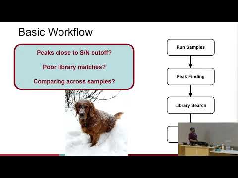
If we look at the basic workflow many people still use, it is something like this: run the samples, perform peak finding for each sample, run library searches, and then generate a peak table. But very quickly, problems appear. What do we do with peaks near the signal-to-noise cutoff? What about peaks with poor library matches? And how do we reconcile all the different peak tables across many samples?

A lot of groups are developing custom solutions, and some of these are now appearing in commercial software. But one thing I wanted for my students — most of whom do not want to code — was a workflow that uses the tools already available in the software, without requiring special scripts from scratch.

The workflow we’ve increasingly adopted relies on retention indices and the IGS peak identification grading system available in the LECO high-resolution workflow. The idea is simple: along with our samples, we run an n-alkane standard to calibrate the retention index method. That allows us to calculate experimental retention indices for all peaks. We can then filter library hits using retention index agreement, and further filter the results by retaining only peaks with good IGS scores, for example scores of 3 or better.

This approach dramatically improves the quality of the peak table. In one pea sample, for example, a standard workflow gave us around 800 peaks, many of which had poor library matches or no useful retention index information. After applying retention index filtering and IGS scoring, that was reduced to 146 peaks that we could be reasonably confident about. The process is automated and straightforward.

This also reveals one of the main issues in complex mixtures: isomers. For example, in a petroleum sample, several alkylbenzenes may all receive slightly different names across different samples, despite being the same underlying feature. This creates a major problem when trying to align peak tables. You may see the same compound identified as 1,2,3-trimethylbenzene in one sample, 1,2,4-trimethylbenzene in another, and something else in a third.

The retention index plus IGS strategy already helps a lot, but it still struggles with some isomeric cases and does not solve everything. In particular, it doesn’t address what I call unknown knowns: peaks that we see repeatedly, expect to be present, but still cannot identify definitively.

To deal with this, we began building a custom mass spectral library, including spectra of standards, local retention index values, and these unknown but recurring peaks. If a compound is well-behaved chromatographically, has a good signal-to-noise ratio, appears in multiple technical replicates or samples, and has a reproducible retention index, we add it to the library. Even if we do not know exactly what it is, we can still assign it a unique code and track it consistently.

That is important. A peak does not need to have a final chemical identity to be useful. If it shows up every time, we can give it a placeholder name and ensure it is always recognized consistently. If it becomes important later, we can return to it and identify it properly.

Once we started using our own custom library with locally measured retention indices, things improved significantly. We obtained more confident high-quality identifications, more peaks with reliable retention index data, and much smaller retention index errors. More importantly, it became very easy to identify the problem peaks — the few peaks that still needed correction because they were likely isomers or misassigned features.

By inspecting retention index deviations, we could quickly spot where the software had assigned the wrong identity. Instead of manually reviewing everything, we could focus only on the handful of peaks that truly required attention. Correcting those few peaks made the retention index agreement even tighter.

Another major advantage of the custom library is that it improves consistency across samples. Peaks that previously received random names or numeric codes from the general NIST search now receive the same identity in every sample, making alignment and downstream chemometric analysis far easier.

So, the main message is this: build your own MS library, include retention index data collected on your own system, and search that first. That allows you to apply a much tighter retention index window and improves confidence in isomer assignments. Also, add your recurring unknown peaks — call them whatever you want, even “Bob” if necessary — so they can be recognized consistently across your dataset.

Apply IGS filtering when possible. If you are not using the same high-resolution workflow, you can still implement similar logic in other software or with simple scripts. The result is better peak tables in less time, more reliable chemometric analysis, and much less manual data curation.

And one final point: learning a bit of Excel automation or simple coding is extremely helpful. It can save a great deal of time when working through these data-heavy workflows.

With that, I’d like to thank LECO for their support with instrumentation and software, our major funders, and the students in the lab working on the Arctic oil and plant volatile projects.

This text has been automatically transcribed from a video presentation using AI technology. It may contain inaccuracies and is not guaranteed to be 100% correct.